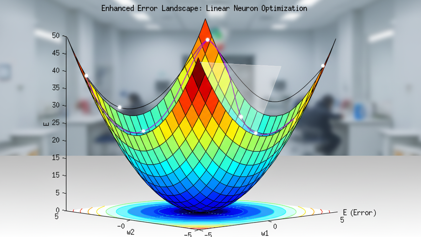
Backpropagation, Gradients, and Computational Graphs

Most modern machine learning systems learn with the same tool. Architectures vary, data differs, and objectives change, yet the training loop is remarkably consistent: compute a loss, propagate gradients, adjust parameters. This uniformity is both the strength of the field and a design constraint developers must respect. In this piece I describe backpropagation as a disciplined way to move information through a differentiable program and highlight the design implications that matter in practice.

Terms and sequence

Model: a function ŷ = f(x; k) with inputs x and parameters k.
Parameters: tunable numbers k = (k0, k1, …); training updates them.
Loss: a scalar L(k) measuring how poorly the model fits the task.
Derivative: local rate of change; for one variable, dL/dk.
Partial derivative: rate of change with respect to one variable while others are held fixed, ∂L/∂k_j.
Gradient: vector of partials ∇L(k) = (∂L/∂k_0, …); points uphill.
Learning rate: a small step size η that scales updates.
Forward pass: compute L from inputs and current parameters.
Backward pass: compute ∇L by applying the chain rule over the program’s computation graph.

This vocabulary is enough to reason about most training systems.

A concrete starting point: curve fitting

Consider a simple approximation problem. We have points (x_i, y_i) and want a smooth function that predicts y from x. One practical choice is a degree-5 polynomial:

ŷ(x) = k0 + k1 x + k2 x^2 + k3 x^3 + k4 x^4 + k5 x^5

Define the loss as the sum of squared errors:

L(k) = Σ_i (y_i − ŷ(x_i))^2

The objective is to find k* = argmin_k L(k).

Two observations shape the solution:

Optimization target: L depends only on the parameters when the data is fixed.
Direction information: if we know the gradient, we know how to change k to reduce L.

Gradient descent in one look

Gradient descent updates parameters in the opposite direction of the gradient:

k ← k − η ∇L(k)

For the polynomial, the partial derivative has a useful structure:

∂L/∂k_j = Σ_i −2 (y_i − ŷ(x_i)) · x_i^j

This pattern repeats across many models: a residual term (y − ŷ) multiplied by a feature term, summed over the dataset.

Why backpropagation?

For simple models we can derive gradients by hand. Real models compose many operations: matrix multiplies, nonlinearities, normalizations, and joins of intermediate results. Hand derivation becomes error-prone.

Backpropagation is a systematic application of the chain rule over a computation graph. It lets us compute ∇L for any program built from differentiable primitives.

Computation graphs and the chain rule

Think of the forward pass as a directed acyclic graph where nodes are values and edges apply operations. The loss L sits at the right; data and parameters sit at the left. Each edge is one of a small set of well-understood operations: add, multiply, power, log, exp, matrix multiply, activation.

The chain rule tells us how to move sensitivities backward through each operation.

Addition: if C = A + B, then ∂L/∂A = ∂L/∂C and ∂L/∂B = ∂L/∂C.
Multiplication: if C = A * B, then ∂L/∂A = (∂L/∂C) · B and ∂L/∂B = (∂L/∂C) · A.
Power (square): if C = A^2, then ∂L/∂A = (∂L/∂C) · 2A.
Split/merge: when a value feeds multiple branches, add the gradients from each branch.

By applying these local rules in reverse topological order, we obtain ∂L/∂k_j for every parameter k_j.

Tiny worked example

# Forward
z = a * b
c = z + d
L = c^2

# Backward
∂L/∂L = 1
∂L/∂c = 2c
∂L/∂z = ∂L/∂c * 1
∂L/∂d = ∂L/∂c * 1
∂L/∂a = ∂L/∂z * b
∂L/∂b = ∂L/∂z * a

The pattern scales. Replace scalars with vectors and matrices and the rules hold with appropriate linear algebra.

A minimal gradient descent sketch

The following sketch shows a plain polynomial fit with an explicit gradient. It is intentionally small to communicate the pattern.

import numpy as np

def poly_predict(x, k):
    # k: shape (6,)
    powers = np.vstack([x**j for j in range(6)])  # shape (6, N)
    return (k[:, None] * powers).sum(axis=0)      # shape (N,)

def poly_gradients(x, y, k):
    y_hat = poly_predict(x, k)
    residual = (y - y_hat)                        # shape (N,)
    grads = np.array([-2 * (residual * (x ** j)).sum() for j in range(6)])
    return grads, (residual**2).sum()

def fit_poly(x, y, steps=2000, lr=1e-3):
    k = np.zeros(6)
    for _ in range(steps):
        g, loss = poly_gradients(x, y, k)
        k -= lr * g
    return k

Replace poly_* with your model’s forward pass and gradients (or let an autodiff engine produce g), keep the loop, and you have the training core.

Design implications for engineers

Backpropagation is not only a math fact; it shapes how we design systems.

Differentiability as a design constraint
- Prefer operations with well-behaved derivatives.
- Avoid discrete choices in the forward path (e.g., argmax); use smooth relaxations (e.g., softmax) when training requires gradients.
- If you must use nondifferentiable steps, isolate them after the loss or use surrogate gradients.
Numerical stability
- Saturating activations slow learning; prefer non-saturating variants or combine with normalization.
- Keep values in safe ranges (e.g., logsumexp for stability, clipping for extreme values).
- Initialization and normalization (LayerNorm, BatchNorm) improve gradient flow.
Step size and schedules
- The learning rate η trades speed for stability. Too small: slow. Too large: divergence.
- Schedules (cosine decay, warmup) and adaptive optimizers (Adam, Adagrad) change the effective step size but preserve the backprop structure.
Batching and vectorization
- Compute losses and gradients over minibatches to reduce variance and exploit hardware.
- Write the forward pass in terms of batched primitives; the backward pass becomes fast for free.
Observability
- Inspect gradient norms by layer. Exploding signals suggest clipping; vanishing suggests architectural or initialization changes.
- Plot the loss across steps. Plateaus often imply poor step size or ill-conditioned geometry.
Memory vs. compute
- Backprop stores intermediates for the backward pass. On large models, this dominates memory use.
- Techniques such as gradient checkpointing trade extra compute for lower memory by recomputing parts of the forward during backward.
Interfaces and boundaries
- Cleanly separate model definition, loss computation, optimizer step, and data pipeline.
- When composing modules, prefer pure functions with explicit inputs/outputs so the graph remains transparent to autodiff.

When backprop struggles

Discontinuities: hard thresholding and data-dependent control flow can make gradients zero or undefined. Use smooth approximations during training.
Poor conditioning: narrow valleys slow descent. Normalization, skip connections, and second-order preconditioning (approximate) improve progress.
Long dependency chains: recurrent computations exacerbate vanishing/exploding gradients. Use gating (LSTM/GRU), residual paths, or attention.
Objective mismatch: if the loss does not reflect the true goal, the gradients point in the wrong direction. Design the loss to encode the real trade-offs.

A short checklist

Define f(x; k) and a single scalar L.
Ensure all forward primitives are differentiable and numerically stable.
Confirm gradients by finite differences on a small problem.
Monitor loss, gradient norms, and a task metric.
Start with a conservative η, then tune.

Closing reflection

Backpropagation is a disciplined way to push information about error through a program. It rewards designs that are explicit, differentiable, and well-conditioned. The trade-off space is familiar: speed vs. stability, expressiveness vs. gradient quality, memory vs. compute. The algorithm stays the same; the craft is in building models—and losses—that give it the right surface to descend.